Streaming Pipelines for Fine-tuning LLMs and RAG in Real-Time
In the 4th lesson, we will focus on the feature pipeline.
The feature pipeline is the first pipeline presented in the 3 pipeline architecture: feature, training and inference pipelines.
A feature pipeline is responsible for taking raw data as input, processing it into features, and storing it in a feature store, from which the training & inference pipelines will use it.
The component is completely isolated from the training and inference code. All the communication is done through the feature store.
To avoid repeating myself, if you are unfamiliar with the 3 pipeline architecture, check out Lesson 1 for a refresher.
By the end of this article, you will learn to design and build a production-ready feature pipeline that:
- uses Bytewax as a stream engine to process data in real-time;
- ingests data from a RabbitMQ queue;
- uses SWE practices to process multiple data types: posts, articles, code;
- cleans, chunks, and embeds data for LLM fine-tuning and RAG;
- loads the features to a Qdrant vector DB.
Note: In our use case, the feature pipeline is also a streaming pipeline, as we use a Bytewax streaming engine. Thus, we will use these words interchangeably.
We will wrap up Lesson 4 by showing you how to deploy the feature pipeline to AWS and integrate it with the components from previous lessons: data collection pipeline, MongoDB, and CDC.
In the 5th lesson, we will go through the vector DB retrieval client, where we will teach you how to query the vector DB and improve the accuracy of the results using advanced retrieval techniques.
Excited? Let’s get started!
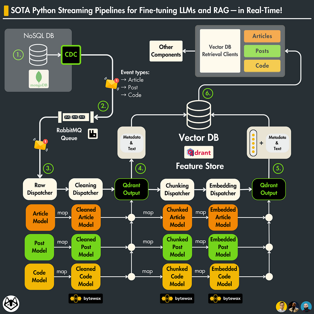
Table of Contents
- Why are we doing this?
- System design of the feature pipeline
- The Bytewax streaming flow
- Pydantic data models
- Load data to Qdrant
- The dispatcher layer
- Preprocessing steps: Clean, chunk, embed
- The AWS infrastructure
- Run the code locally
- Deploy the code to AWS & Run it from the cloud
- Conclusion
🔗 Check out the code on GitHub [1] and support us with a ⭐️
1. Why are we creating a streaming pipeline?
A quick reminder from previous lessons
To give you some context, in Lesson 2, we crawl data from LinkedIn, Medium, and GitHub, normalize it, and load it to MongoDB.
In Lesson 3, we are using CDC to listen to changes to the MongoDB database and emit events in a RabbitMQ queue based on any CRUD operation done on MongoDB.
…and here we are in Lesson 4, where we are building the feature pipeline that listens 24/7 to the RabbitMQ queue for new events to process and load them to a Qdrant vector DB.
The problem we are solving
In our LLM Twin use case, the feature pipeline constantly syncs the MongoDB warehouse with the Qdrant vector DB while processing the raw data into features.
Important: In our use case, the Qdrant vector DB will be our feature store.
Why we are solving it
The feature store will be the central point of access for all the features used within the training and inference pipelines.
For consistency and simplicity, we will refer to different formats of our text data as “features.”
→ The training pipeline will use the feature store to create fine-tuning datasets for your LLM twin.
→ The inference pipeline will use the feature store for RAG.
For reliable results (especially for RAG), the data from the vector DB must always be in sync with the data from the data warehouse.
The question is, what is the best way to sync these 2?
Other potential solutions
The most common solution is probably to use a batch pipeline that constantly polls from the warehouse, computes a difference between the 2 databases, and updates the target database.
The issue with this technique is that computing the difference between the 2 databases is extremely slow and costly.
Another solution is to use a push technique using a webhook. Thus, on any CRUD change in the warehouse, you also update the source DB.
The biggest issue here is that if the webhook fails, you have to implement complex recovery logic.
Lesson 3 on CDC covers more of this.
2. System design of the feature pipeline: our solution
Our solution is based on CDC, a queue, a streaming engine, and a vector DB:
→ CDC adds any change made to the Mongo DB to the queue (read more in Lesson 3).
→ the RabbitMQ queue stores all the events until they are processed.
→ The Bytewax streaming engine cleans, chunks, and embeds the data.
→ A streaming engine works naturally with a queue-based system.
→ The data is uploaded to a Qdrant vector DB on the fly
Why is this feature pipeline design powerful?
Here are 4 core reasons:
- The data is processed in real-time.
- Out-of-the-box recovery system: If the streaming pipeline fails to process a message will be added back to the queue
- Lightweight: No need for any diffs between databases or batching too many records
- No I/O bottlenecks on the source database
→ It solves all our problems!
How is the data stored in our streaming pipeline?
We store 2 snapshots of our data in the feature store. Here is why ↓
Remember that we said that the training and inference pipeline will access the features only from the feature store, which, in our case, is the Qdrant vector DB?
Well, if we had stored only the chunked & embedded version of the data, that would have been useful only for RAG but not for fine-tuning.
Thus, we make an additional snapshot of the cleaned data, which will be used by the training pipeline.
Afterward, we pass it down the streaming flow for chunking & embedding.
How do we process multiple data types for our feature pipeline?
How do you process multiple types of data in a single streaming pipeline without writing spaghetti code?
Yes, that is for you, data scientists! Joking…am I?
We have 3 data types: posts, articles, and code.
Each data type (and its state) will be modeled using Pydantic models.
To process them we will write a dispatcher layer, which will use a creational factory pattern [9] to instantiate a handler implemented for that specific data type (post, article, code) and operation (cleaning, chunking, embedding).
The handler follows the strategy behavioral pattern [10].
Intuitively, you can see the combination between the factory and strategy patterns as follows:
- Initially, we know we want to clean the data, but as we don’t know the data type, we can’t know how to do so.
- What we can do, is write the whole code around the cleaning code and abstract away the login under a Handler() interface (aka the strategy).
- When we get a data point, the factory class creates the right cleaning handler based on its type.
- Ultimately the handler is injected into the rest of the system and executed.
By doing so, we can easily isolate the logic for a given data type & operation while leveraging polymorphism to avoid filling up the code with 1000x “if else” statements.
We will dig into the implementation in future sections.
Streaming over batch in our pipeline
You may ask why we need a streaming engine instead of implementing a batch job that polls the messages at a given frequency.
That is a valid question.
The thing is that…
Nowadays, using tools such as Bytewax makes implementing streaming pipelines a lot more frictionless than using their JVM alternatives.
The key aspect of choosing a streaming vs. a batch design is real-time synchronization between your source and destination DBs.
In our particular case, we will process social media data, which changes fast and irregularly.
Also, for our digital twin, it is important to do RAG on up-to-date data. We don’t want to have any delay between what happens in the real world and what your LLM twin sees.
That being said choosing a streaming architecture seemed natural in our use case.
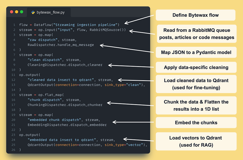
3. The Bytewax streaming flow for a feature pipeline
The Bytewax flow is the central point of the streaming pipeline. It defines all the required steps, following the next simplified pattern: “input -> processing -> output”.
As I come from the AI world, I like to see it as the “graph” of the streaming pipeline, where you use the input(), map(), and output() Bytewax functions to define your graph, which in the Bytewax world is called a “flow”.
As you can see in the code snippet below, we ingest posts, articles or code messages from a RabbitMQ queue. After we clean, chunk and embed them. Ultimately, we load the cleaned and embedded data to a Qdrant vector DB, which in our LLM twin use case will represent the feature store of our system.
To structure and validate the data, between each Bytewax step, we map and pass a different Pydantic model based on its current state: raw, cleaned, chunked, or embedded.
We have a single streaming pipeline that processes everything.
As we ingest multiple data types (posts, articles, or code snapshots), we have to process them differently.
To do this the right way, we implemented a dispatcher layer that knows how to apply data-specific operations based on the type of message.
More on this in the next sections ↓
Why Bytewax for our feature pipeline?
Bytewax is an open-source streaming processing framework that:
– is built in Rust ⚙️ for performance
– has Python 🐍 bindings for leveraging its powerful ML ecosystem
… so, for all the Python fanatics out there, no more JVM headaches for you.
Jokes aside, here is why Bytewax is so powerful ↓
– Bytewax local setup is plug-and-play
– can quickly be integrated into any Python project (you can go wild — even use it in Notebooks)
– can easily be integrated with other Python packages (NumPy, PyTorch, HuggingFace, OpenCV, SkLearn, you name it)
– out-of-the-box connectors for Kafka and local files, or you can quickly implement your own
We used Bytewax to build the streaming pipeline for the LLM Twin course and loved it.
To learn more about Bytewax, go and check them out. They are open source, so no strings attached → Bytewax [2] ←
4. Pydantic data models
Let’s take a look at what our Pydantic models look like.
First, we defined a set of base abstract models for using the same parent class across all our components.
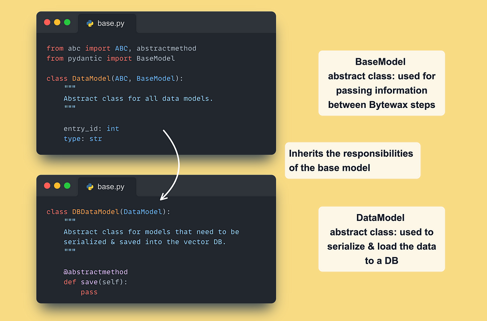
Afterward, we defined a hierarchy of Pydantic models for:
- all our data types: posts, articles, or code
- all our states: raw, cleaned, chunked, and embedded
This is how the set of classes for the posts will look like ↓
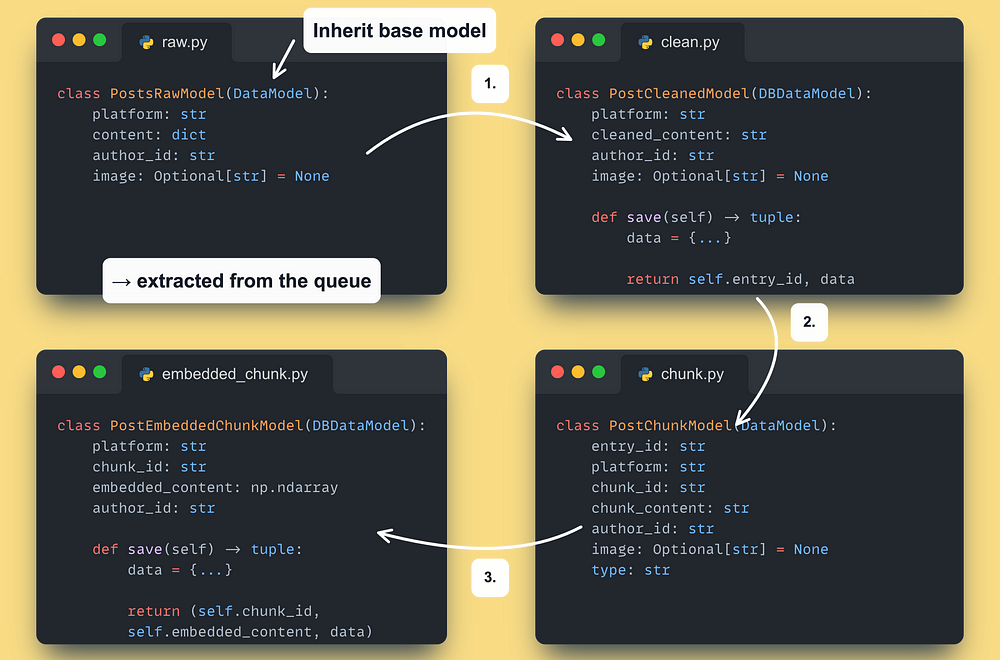
We repeated the same process for the articles and code model hierarchy.
Check out the other data classes on our GitHub.
Why is keeping our data in Pydantic models so powerful?
There are 4 main criteria:
- every field has an enforced type: you are ensured the data types are going to be correct
- the fields are automatically validated based on their type: for example, if the field is a string and you pass an int, it will through an error
- the data structure is clear and verbose: no more clandestine dicts that you never know what is in them
- you make your data the first-class citizen of your program
5. Load data to Qdrant
The first step is to implement our custom Bytewax DynamicSink class ↓
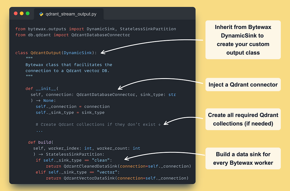
Next, for every type of operation we need (output cleaned or embedded data ) we have to subclass the StatelessSinkPartition Bytewax class (they also provide a stateful option → more in their docs)
An instance of the class will run on every partition defined within the Bytewax deployment.
In the course, we are using a single partition per worker. But, by adding more partitions (and workers), you can quickly scale your Bytewax feature pipeline horizontally.
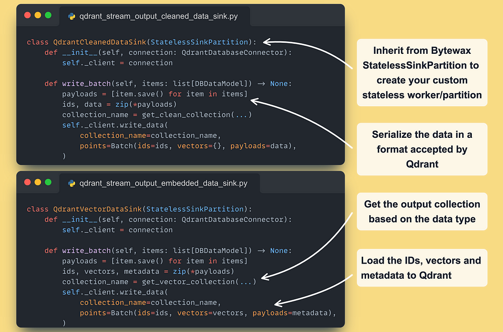
Note that we used Qdrant’s Batch method to upload all the available points at once. By doing so, we reduce the latency on the network I/O side: more on that here [8] ←
The RabbitMQ streaming input follows a similar pattern. Check it out here ←
6. The dispatcher layer
Now that we have the Bytewax flow and all our data models.
How do we map a raw data model to a cleaned data model?
→ All our domain logic is modeled by a set of Handler() classes.
For example, this is how the handler used to map a PostsRawModel to a PostCleanedModel looks like ↓
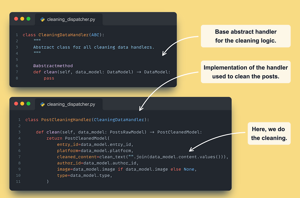
Check out the other handlers on our GitHub:
In the next sections, we will explore the exact cleaning, chunking and embedding logic.
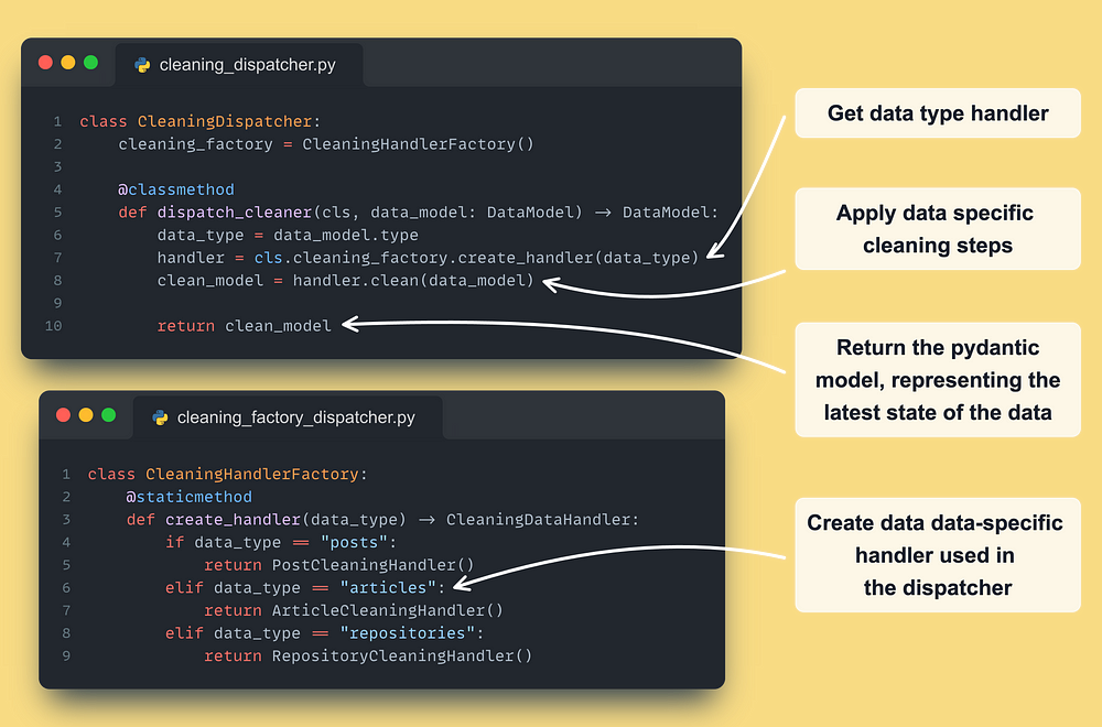
Now, to build our dispatcher, we need 2 last components:
- a factory class: instantiates the right handler based on the type of the event
- a dispatcher class: the glue code that calls the factory class and handler
Here is what the cleaning dispatcher and factory look like ↓
Check out the other dispatchers on our GitHub.
By repeating the same logic, we will end up with the following set of dispatchers:
- RawDispatcher (no factory class required as the data is not processed)
- CleaningDispatcher (with a ChunkingHandlerFactory class)
- ChunkingDispatcher (with a ChunkingHandlerFactory class)
- EmbeddingDispatcher (with an EmbeddingHandlerFactory class)
7. Preprocessing steps: Clean, chunk, embed
Here we will focus on the concrete logic used to clean, chunk, and embed a data point.
Note that this logic is wrapped by our handler to be integrated into our dispatcher layer using the Strategy behavioral pattern [10].
We already described that in the previous section. Thus, we will directly jump into the actual logic here, which can be found in the utils module of our GitHub repository.
Note: These steps are experimental. Thus, what we present here is just the first iteration of the system. In a real-world scenario, you would experiment with different cleaning, chunking or model versions to improve it on your data.
Cleaning
This is the main utility function used to clean the text for our posts, articles, and code.
Out of simplicity, we used the same logic for all the data types, but after more investigation, you would probably need to adapt it to your specific needs.
For example, your posts might start containing some weird characters, and you don’t want to run the “unbold_text()” or “unitalic_text()” functions on your code data point as is completely redundant.
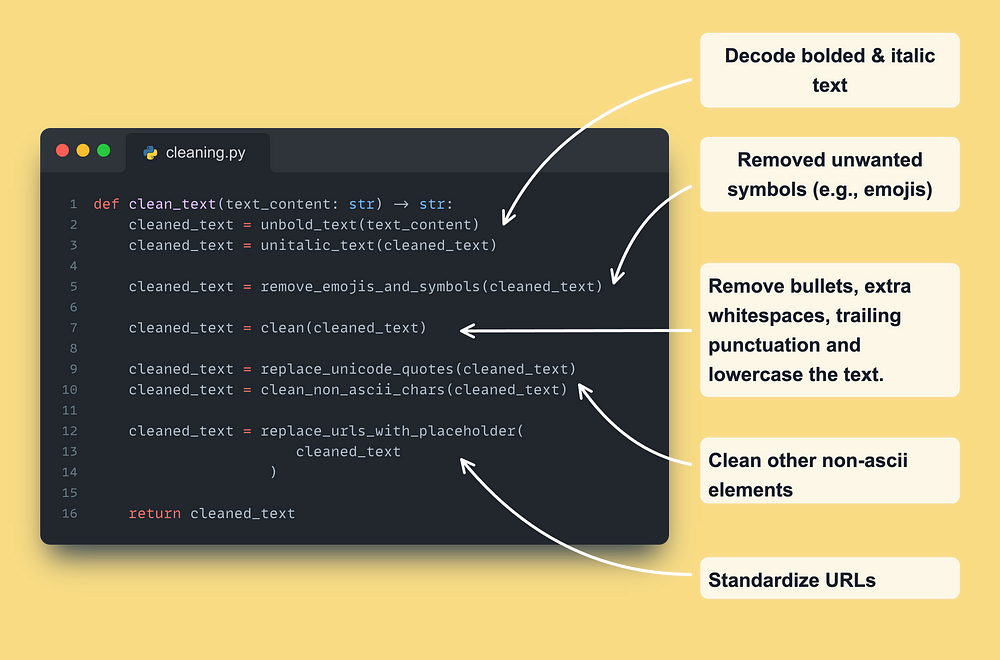
Most of the functions above are from the unstructured [3] Python package. It is a great tool for quickly finding utilities to clean text data.
🔗 More examples of unstructured here [3] ←
One key thing to notice is that at the cleaning step, we just want to remove all the weird, non-interpretable characters from the text.
Also, we want to remove redundant data, such as extra whitespace or URLs, as they do not provide much value.
These steps are critical for our tokenizer to understand and efficiently transform our string input into numbers that will be fed into the transformer models.
Note that when using bigger models (transformers) + modern tokenization techniques, you don’t need to standardize your dataset too much.
For example, it is redundant to apply lemmatization or stemming, as the tokenizer knows how to split your input into a commonly used sequence of characters efficiently, and the transformers can pick up the nuances of the words.
💡 What is important at the cleaning step is to throw out the noise.
Chunking
We are using Langchain to chunk our text.
We use a 2 step strategy using Langchain’s RecursiveCharacterTextSplitter [4] and SentenceTransformersTokenTextSplitter [5]. As seen below ↓
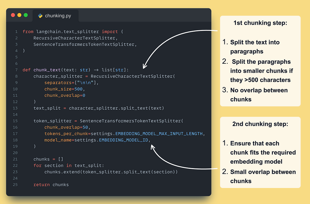
Overlapping your chunks is a common pre-indexing RAG technique, which helps to cluster chunks from the same document semantically.
Again, we are using the same chunking logic for all of our data types, but to get the most out of it, we would probably need to tweak the separators, chunk_size, and chunk_overlap parameters for our different use cases.
But our dispatcher + handler architecture would easily allow us to configure the chunking step in future iterations.
Embedding
The data preprocessing, aka the hard part is done.
Now we just have to call an embedding model to create our vectors.
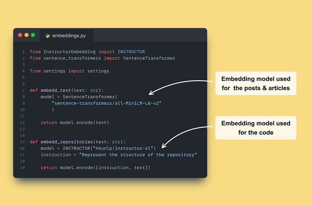
We used the all-MiniLm-L6-v2 [6] from the sentence-transformers library to embed our articles and posts: a lightweight embedding model that can easily run in real-time on a 2 vCPU machine.
As the code data points contain more complex relationships and specific jargon to embed, we used a more powerful embedding model: hkunlp/instructor-xl [7].
This embedding model is unique as it can be customized on the fly with instructions based on your particular data. This allows the embedding model to specialize on your data without fine-tuning, which is handy for embedding pieces of code.
8. The AWS infrastructure
In Lesson 2, we covered how to deploy the data collection pipeline that is triggered by a link to Medium, Substack, LinkedIn or GitHub → crawls the given link → saves the crawled information to a MongoDB.
In Lesson 3, we explained how to deploy the CDC components that emit events to a RabbitMQ queue based on any CRUD operation done to MongoDB.
What is left is to deploy the Bytewax streaming pipeline and Qdrant vector DB.
We will use Qdrant’s self-hosted option, which is easy to set up and scale.
To test things out, they offer a Free Tier plan for up to a 1GB cluster, which is more than enough for our course.
→ We explained in our GitHub repository how to configure Qdrant.
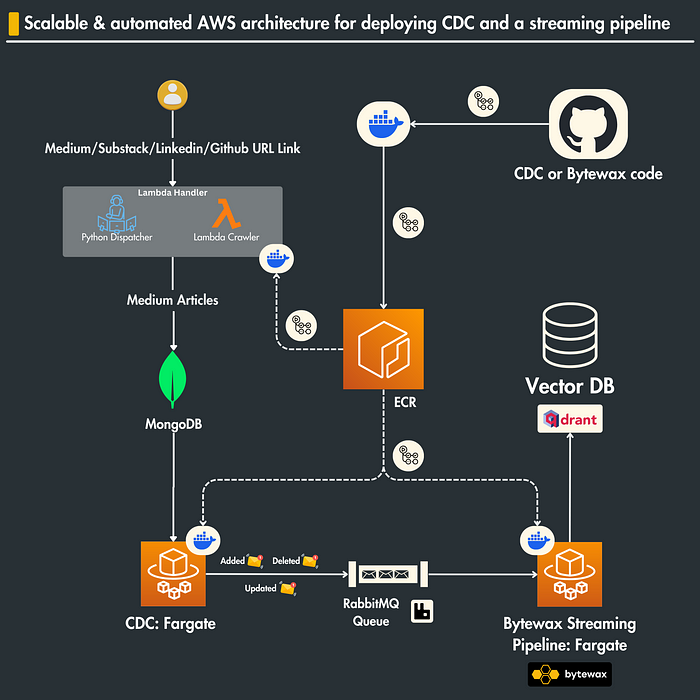
The last piece of the puzzle is the Bytewax streaming pipeline.
As we don’t require a GPU and the streaming pipeline needs to run 24/7, we will deploy it to AWS Fargate, a cost-effective serverless solution from AWS.
As a serverless solution, Fargate allows us to deploy our code quickly and scale it fast in case of high traffic.
How do we deploy the streaming pipeline code to Fargate?
Using GitHub Actions, we wrote a CD pipeline that builds a Docker image on every new commit made on the main branch.
After, the Docker image is pushed to AWS ECR. Ultimately, Fargate pulls the latest version of the Docker image.
This is a common CD pipeline to deploy your code to AWS services.
Why not use lambda functions, as we did for the data pipeline?
An AWS lambda function executes a function once and then closes down.
This worked perfectly for the crawling logic, but it won’t work for our streaming pipeline, which has to run 24/7.
9. Run the code locally
To quickly test things up, we wrote a docker-compose.yaml file to spin up the MongoDB, RabbitMQ queue and Qdrant vector db.
You can spin up the Docker containers using our Makefile by running the following:
make local-start-infra
To fully test the Bytewax streaming pipeline, you have to start the CDC component by running:
make local-start-cdc
Ultimately, you start the streaming pipeline:
make local-bytewax
To simulate the data collection pipeline, mock it as follows:
make local-insert-data-mongo
The README of our GitHub repository provides more details on how to run and set up everything.
10. Deploy the code to AWS & Run the streaming pipeline from the cloud
This article is already too long, so I won’t go into the details of how to deploy the AWS infrastructure described above and test it out here.
But to give you some insights, we have used Pulumi as our infrastructure as a code (IaC) tool, which will allow you to spin it quickly with a few commands.
Also, I won’t let you hang on to this one. We made a promise and… ↓
We prepared step-by-step instructions in the README of our GitHub repository on how to use Pulumni to spin up the infrastructure and test it out.
Conclusion
Now you know how to write streaming pipelines like a PRO!
In Lesson 4, you learned how to:
- design a feature pipeline using the 3-pipeline architecture
- write a streaming pipeline using Bytewax as a streaming engine
- use a dispatcher layer to write a modular and flexible application to process multiple types of data (posts, articles, code)
- load the cleaned and embedded data to Qdrant
- deploy the streaming pipeline to AWS
→ This is only the ingestion part used for fine-tuning LLMs and RAG.
In Lesson 5, you will learn how to write a retrieval client for the 3 data types using good SWE practices and improve the retrieval accuracy using advanced retrieval & post-retrieval techniques. See you there!
🔗 Check out the code on GitHub [1] and support us with a ⭐️
Related Articles